Excel · Google Sheets · pivot
Excel percentage formulas – ready formulas to copy
Pick a calculation and the cells, and you get a ready formula for Excel and Google Sheets. It also covers pivot-table percentage views and the cell-formatting pitfalls that trip people up.
Your recent calculations
Calculations are saved only in this browser (localStorage). They are not sent to the server and we cannot see them.
Percentage formulas in a spreadsheet
| Situation | Excel / Sheets |
|---|---|
| A as a % of B | =A2/B2 |
| Change from old to new | =(B2-A2)/A2 |
| B % of the number A | =A2*B2 |
| Price −X% | =A2*(1-B2) |
| Price +X% | =A2*(1+B2) |
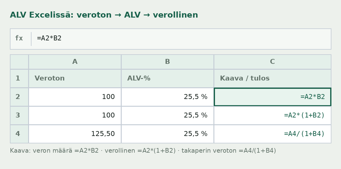
| Net price from a gross one | =A2/(1+B2) |
| Share of the total | =A2/SUM($A$2:$A$100) |
| Error handling | =IFERROR(A2/B2,0) |
| Round to four decimals | =ROUND(A2/B2,4) |
The separator depends on your settings. In Google Sheets and English (UK/US)
settings, function arguments are separated by a comma (,). Some regional Windows setups use a semicolon
(;) because the comma is the decimal separator. If a formula errors the moment you paste it, this is
almost always why.
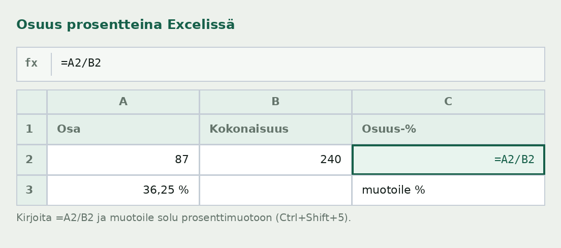
Why the result shows 0.25 instead of 25%
Excel works out a percentage as a decimal. The formula =A2/B2 returns 0.25, which
is 25% – the cell just shows it in the wrong format. You fix it with formatting, not by multiplying by
a hundred.
- Select the cell or range.
- Home tab → Number group → percentage format (
%) or Ctrl+Shift+%. - Adjust the number of decimals with the arrow buttons.
If you multiply the formula by a hundred and apply percentage formatting, you get 2,500% – the classic double-up. So pick one: either the formatting or multiplying by a hundred without the percent sign.
Pivot-table percentage views
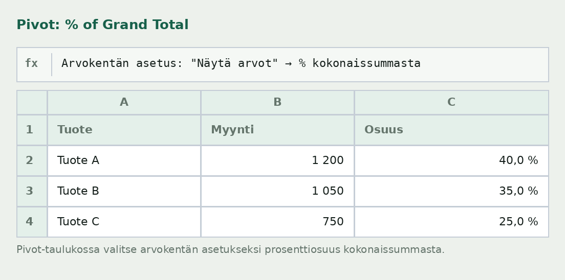
In a pivot table you don't work out a percentage with a formula – you choose a display setting. This is faster and updates automatically when the source data changes.
- Right-click a value field in the pivot table.
- Choose Show Values As.
- Pick the view you want:
- % of Grand Total – the row's share of the whole table's total.
- % of Row Total – the cell's share of its own row's total.
- % of Column Total – the cell's share of its own column's total.
- % of Parent Total – a comparison to a chosen base value.
- % Difference From – the growth against the previous period.
- If you like, add the same field twice: one in pounds, one as a percentage.
A conditional percentage
Often you need a share of just one group: how much one salesperson's deals are of total sales, or what share of orders came from a particular region. Then the numerator is a conditional sum.
| Need | Excel / Sheets |
|---|---|
| One group's share of the total | =SUMIF($A$2:$A$100,D2,$B$2:$B$100)/SUM($B$2:$B$100) |
| Share of rows meeting a condition | =COUNTIF($A$2:$A$100,"Yes")/COUNTA($A$2:$A$100) |
| Share on two conditions | =SUMIFS(...)/SUM($B$2:$B$100) |
Remember absolute references with the dollar sign ($B$2:$B$100). Without them, the sum range shifts
when you copy the formula down, and the percentages go wrong without you noticing.
Highlighting percentages with conditional formatting
When a table has dozens of percentage rows, it's better to bring out the outliers with formatting than by eye.
- Select the percentage column.
- Home → Conditional Formatting.
- Colour Scales show the ranking with a gradient, Data Bars draw a bar in the cell, and Icon Sets add up or down arrows.
- Make negative changes red with the rule Cell Value < 0.
For change percentages, an icon set is clearest: the reader sees at a glance what grew and what fell, without having to read every number separately.
The most common error messages
| Error | Cause | Fix |
|---|---|---|
#DIV/0! | The divisor is zero or empty | Wrap the formula: =IFERROR(A2/B2,0) |
#VALUE! | The cell contains text, e.g. "25%" as text | Convert to a number or remove the unit from the cell |
#NAME? | The function name is spelled wrong or in the wrong language | Use SUM, IFERROR etc. in English |
| The formula shows as text | The cell is formatted as text | Change the format to General and re-enter the formula |
The basics of spreadsheet percentages
Excel works out a percentage as a decimal. The display is fixed with cell formatting, not by multiplying by a hundred.
Formulas and examples
Share of the total
=A2/B2Example
The result 0.25 shows as 25% when formatted as a percentage.
Note
If you also multiply by a hundred and format as a percentage, you get 2,500%.
Percentage change
=(B2-A2)/A2Example
A2 = old, B2 = new. A negative result means a decrease.
Note
Format the cell as a percentage with 0–2 decimals.
Net price from a gross one
=A2/(1+B2)Example
B2 = VAT rate as a percentage, for example 20%.
Note
The same formula works for any rate when B2 is updated.
Error handling
=IFERROR(A2/B2,0)Example
Prevents the #DIV/0! error when the divisor is empty or zero.
Note
In some regional settings the argument separator is a semicolon.
Concepts and classification
| Separator | A comma ( , ) in English/Sheets; a semicolon ( ; ) in some regions. |
|---|---|
| Percentage format | Ctrl + Shift + % – changes only the display. |
| Absolute reference | $B$2 stays put when the formula is copied. |
| Pivot percentage | Show Values As → % of Grand Total. |
| SUMIF | A conditional sum. |
Limitations
- Function names are language-dependent – the wrong language gives a #NAME? error.
- A number stored as text (e.g. "25%") isn't included in the calculation.
- Pivot menu names vary between Excel versions.
- Google Sheets always uses a comma as the separator.
How up to date the information is
When it was checked
Content and the formulas used were checked on 12 August 2026.
Disclaimer
The calculator gives a mathematical result from the numbers you enter. It is not an official decision, an offer or professional advice. See the terms of use.
Topics
This calculator belongs to the following topic areas. On the topic page you'll find all the calculators and guides on the same theme in one place.
Calculators whose formulas you take into Excel
Frequently asked questions about Excel percentage formulas
How do I work out a percentage in Excel?
Use =A2/B2 and format the cell as a percentage. The formula returns a decimal, e.g. 0.25, which shows as 25% once formatted.
Why does Excel show 0.25 instead of 25%?
The cell is in number format. Change it to percentage with Ctrl+Shift+%. Don't multiply the formula by 100 if you're using percentage formatting – otherwise the result is a hundred times too big.
What is the percentage change formula in Excel?
=(B2-A2)/A2, where A2 is the old value and B2 the new one. Format the result as a percentage. A negative result means a decrease.
How do I show percentages of the total in a pivot table?
Right-click the value field, choose Show Values As and then % of Grand Total. You can also choose a percentage of the row or column total.
Do I use a semicolon or a comma inside a function?
Google Sheets and English (UK/US) settings use a comma. Some regional Windows settings use a semicolon because the comma is the decimal separator. The generator gives the formula in both forms.
How do I prevent the #DIV/0! error?
Wrap the division in error handling: =IFERROR(A2/B2,0). The formula returns zero if the divisor is empty or zero.